Basics
The landscape evolution simulations presented on this site have been carried out
using the CIDRE code (e.g. Carretier et al., 2016). This website has not been
created as an apology for CIDRE. There are other freely usable models with
remarkable performances of which a non-exhaustive list is given in the table at the
end of this page. All LEMs applied over millions of years have common points
(stationarity of water flows in most of the cases, general shape of erosion laws) but
also different levels of simplification concerning hydrology and sediment transport
which can vary. Some algorithms are frighteningly fast, while others favour the
addition of certain processes (e.g. lateral erosion in CIDRE). A feature of CIDRE
that exists in few models is its ability to ”spread” water runoff (Multiple flow
algorithm instead of steepest descent algorithm), which can therefore diverge
and more realistically account for the flow over foothills and plain areas.
In CIDRE, topography is represented by a mesh of square cells (or pixels). Each
cell has an altitude and a constant size. Basically, CIDRE is injected with a rain grid
or a constant value, an initial topography, a tectonic uplift rate grid or value, an erodibility grid
or a value and CIDRE calculates over time the evolution of the topography, the
quantity eroded or the quantity of sediments deposited on every cell of the
grid.
In practice, over a time step (about 100 years), CIDRE runs the cells in the
decreasing direction of the altitudes. It propagates the quantity of water fallen
by the rain to calculate a water discharge flowing on each cell, and it also
calculates the slopes between this cell and its lower neighbours. From the
steepest slope and from the water discharge CIDRE calculates the amount
that can be eroded, and the amount of moving sediment from higher up
that will be deposited. In addition, the water flow can erode the lateral
neighbours cells (bank erosion). Eroded and transiting material is transferred to
the lower cells in proportion to the slope. Then CIDRE moves to the cell
that is lower in the list and so on until all the cells have been treated. An
increment of tectonic uplit is added to elevations. Then a new time step starts
and the same process is repeated until the total duration of the model is
reached.
Equations
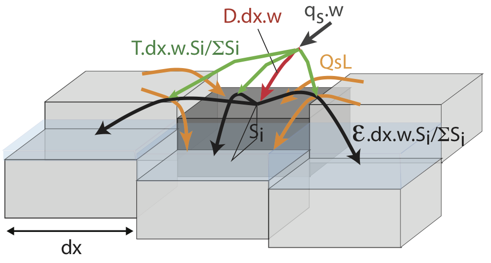
Starting from an initial topography, the modification of the topography proceeds by
successive time steps. During a time step, precipitation falls on the grid at a rate P
[LT-1] and a multiple flow algorithm propagates the water flux Q [L3T-1], toward all
downstream cells in proportion to the slope in each direction. Then the elevation z
(river bed or hillslope surface) changes on each cell (size dx) according to the
balance between erosion ϵ [LT-1] and deposition D [LT-1]. The erosion is
different for sediment and for bedrock and ϵ is the sum of two values, one
corresponding to gravitational processes without involving the runoff, usually
dominating on the hillslopes, and another one associated with water discharge,
typically dominating in rivers. Water flowing in one direction is also able to
detach material from the cells located perpendicular to that direction to
simulate river bank erosion. This erosion generates a lateral (bank) sediment
discharge Qsl [L3T-1] toward the cell where the water is flowing. Finally,
elevation changes also by adding an uplift U [LT-1] (subsidence if negative).
In the following, all the water and sediment fluxes are ”per unit width”
[L2T-1], the width being either a calculated sub-pixel flow width, or the
pixel size dx. All the simulations in this website were run using this second
option.
The rate of elevation change on a cell is determined by the following mass balance equation (e.g. Davy and Lague, 2009; Carretier et al., 2016; Shobe et al., 2017):

where the subscript ”r” (”river”) denotes rates associated with flowing water and ”h” (”hillslope”) denotes rates that depends only on the topographic gradient or slope S. Then we define a constitutive law for each of these components: (Carretier et al., 2016)
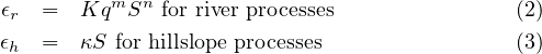
where K [L1-2mTm-1], κ [LT-1] are erodibility parameters, m and n are lithology-dependent (different for bedrock or sediment) erosion parameters, S is the slope, q [L2T-1] is the water discharge per stream unit width, and
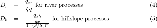
where qsr and qsh are the incoming river and hillslope sediment fluxes (total
qs = qsr + qsh) per unit width [L2T-1], ζ is a river transport length parameter [T
L-1] and Sc is a slope threshold. These fluxes are the sum of sediment fluxes leaving
upstream neighbour cells while the deposition rates on a cell are a fraction of the
incoming sediment.
Concerning the river processes, ϵr is known as the stream power law and derives
from the assumption that ϵr is proportional to a power law of the shear stress applied
by the flowing water on the river bed (e.g. Whipple et al., 2000; Lague, 2014).
The deposition rate Dr is a fraction of the incoming sediment flux and this
fraction (ζq) has the dimension of the reverse of a length. We call this length a
transport length because it has the physical meaning of a characteristic distance
over which a volume of detached material will transit downstream before
being deposited. In particular, when the local q is large, few sediment eroded
from upstream will deposit on the cell. The transport length depends on
ζ, proportional to the reverse of a settling velocity of sediment in water
(e.g. Davy and Lague, 2009; Lajeunesse et al., 2013). In instantaneous river
models, ζ should be fixed by the grain size of sediment. In landscape evolution
models, where the water discharge q averages the periods with and without
transport, ζ is an ”apparent” parameter that can take a large range of values
in real situations depending on climate variability (Guerit et al., 2019).
Concerning the hillslopes processes, the philosophy is the same, except that the
detachment rate ϵr and the deposition rate Dr depend only on the slope. The linear
slope dependence of ϵr describes diffusion processes. Dr depends on a specified
critical slope Sc: when the slope is close to Sc, the deposition rate Dr decreases
rapidly, simulating in average the onset of shallow landslides. The transport length
associated with gravitational processes ( ) is inversely proportional
to the probability to deposit sediment on the cell. This erosion-deposition
formulation leads to similar solutions as the critical slope-dependent hillslope
model studied for example by Roering et al. (1999) (Carretier et al., 2016).
) is inversely proportional
to the probability to deposit sediment on the cell. This erosion-deposition
formulation leads to similar solutions as the critical slope-dependent hillslope
model studied for example by Roering et al. (1999) (Carretier et al., 2016).
Flowing water in each direction can erode lateral cells perpendicular to that direction. Little is known about the law that describes the widening rate of valley, and establishing a lateral erosion law suitable for landscape evolution models averaging processes over millennia is a challenge (Langston and Tucker, 2018; Langston and Temme, 2019). Here, the lateral sediment flux per unit length qsl [L2T-1] eroded from a lateral cell is simply defined as a fraction of the river sediment flux qsr [L2T-1] in the considered direction (e.g. Murray and Paola, 1997; Nicholas and Quine, 2007), assuming that lateral mobility of channels, and thus lateral erosion, increases with the flux of river sediment (Bufe et al., 2016, 2019):

where α is a bank erodibility coefficient. α is specified for loose material
(sediment) and is implicitly determined for bedrock layers such that the
ratio of the lateral erodabilities is equal to the ratio of the fluvial ones
(αloose∕αbedrock = Kloose∕Kbedrock , with K from Equation 2). If sediment covers the
bedrock of a lateral cell, α is weighted by its respective thickness above the target
cell.
Finally, the sediment leaving a cell is spread in the same way as water, i.e.
proportionally to the downstream slopes. This procedures starts from the most
elevated cell and ends with the lowest cell and is repeated in the next time steps until
the end of the specified model time (Myr in our case).
Parameter values for the reference simulation
The reference simulation is a constantly uplifting domain grid of 40x40 km2 (200x200
cells of size 200 m).
Associating erodibility parameters to a particular rock is challenging. The best
that we can do in the current state of our knowledge is to fix the erodibility
parameters so that the relief is realistic. We impose here only one bedrock type for
which the erodibility is K = 10-4 m-0.5 yr-1, and the water discharge and slope
exponent are m = 0.5, n = 1. The bedrock erodibility by pure gravitational processes
is κ = 10-4 m yr-1. For the sediment (previously deposited but that can be
reeroded), we use K = 10-3 m-0.5 yr-1, m = 0.5, n = 1 and κ = 10-4 m yr-1.
The transport length parameter ζ is set to 1 yr m-1, and corresponds to a low
value for natural systems (median at 17 yr/m Guerit et al., 2019). It is difficult to
link ζ with physical properties of sediment because ζ changes according to the
variability of transport periods, but low values seem to correspond to temperate
perennial rivers (Guerit et al., 2019).
The lateral erosion parameter α to 0. Finally, the critical slope is Sc =tan(40o).
The northern southern sides are open and fixed to z = 0 m. Periodic boundary
conditions are imposed on the two other sides meaning that water and sediment
leaving on the one side is reinjected on the other one.
U is fixed to 10-3 m yr-1 and P to 1 m yr-1.
The final time is fixed to 7 Ma for the reference simulation, a duration allowing
the topography to reach a dynamic equilibrium, ie. a state where the topography
does not change in average and the erosion balances uplift. For some simulations, this
time is longer because the topography takes more time to reach a dynamic
equilibrium.
Existing LEMs
| LEM | Reference |
| SIBERIA | |
| DRAINAL | |
| GILBERT | |
| DELIM | |
| GOLEM | |
| CASCADE | |
| CAESAR | |
| ZSCAPE | |
| CHILD | |
| EROS | |
| APERO | |
| CAESAR-LISFLOOD | |
| DAC | |
| CIDRE | |
| TTLEM | |
| Landlab-SPACE | |
| EROS-FLOODOS | |
| FASTSCAPE | |
|
|
References
Beaumont, C., P. Fullsack, and J. Hamilton (1992), Erosional control of active compressional orogens. In K.R. Mc Clay (Ed.), thrust Tectonics, 1-18 pp., Chapman and Hall, New Yotk.
Braun, J., and M. Sambridge (1997), Modelling landscape evolution on geological time scales: a new method based on irregular spatial discretization, Basin Res., 9, 27–52.
Bufe, A., C. Paola, and D. W. Burbank (2016), Fluvial bevelling of topography controlled by lateral channel mobility and uplift rate, Nature Geoscience, 9(9), 706.
Bufe, A., J. M. Turowski, D. W. Burbank, C. Paola, A. D. Wickert, and S. Tofelde (2019), Controls on the lateral channel-migration rate of braided channel systems in coarse non-cohesive sediment, Earth Surf. Proc. Land., 44(14), 2823–2836, doi:10.1002/esp.4710.
Campforts, B., W. Schwanghart, and G. Govers (2017), Accurate simulation of transient landscape evolution by eliminating numerical diffusion: the TTLEM 1.0 model, Earth Surface Dynamics, 5(1), 47–66, doi:10.5194/esurf-5-47-2017.
Carretier, S., and F. Lucazeau (2005), How does alluvial sedimentation at range fronts modify the erosional dynamics of mountain catchments?, Basin Res., 17, 361–381, doi:10.1111/j.1365-2117.2005.00270.x.
Carretier, S., P. Martinod, M. Reich, and Y. Goddéris (2016), Modelling sediment clasts transport during landscape evolution, Earth Surf. Dynam., 4, 237–251, doi:10.5194/esurf-4-237-2016.
Chase, C. G. (1992), Fluvial landsculpting and the fractal dimension of topography, Geomorphology, 5, 39–57.
Coulthard, T., M. Kirkby, and M. Macklin (1998), Non-linearity and spatial resolution in a cellular automaton model of a small upland basin, Hydrology And Earth System Sciences, 2(2-3), 257–264, doi:10.5194/hess-2-257-1998.
Coulthard, T. J., J. C. Neal, P. D. Bates, J. Ramirez, G. A. M. de Almeida, and G. R. Hancock (2013), Integrating the LISFLOOD-FP 2D hydrodynamic model with the CAESAR model: implications for modelling landscape evolution, Earth Surf. Proc. Land., 38(15), 1897–1906, doi:10.1002/esp.3478.
Crave, A., and P. Davy (2001), A stochastic ”precipitation” model for simulating erosion/sedimentation dynamics, Computer and GeoSciences, 27(7), 815–827.
Davy, P., and D. Lague (2009), The erosion / transport equation of landscape evolution models revisited, J. Geophys. Res., 114, doi:10.1029/2008JF001146.
Davy, P., T. Croissant, and D. Lague (2017), A precipiton method to calculate river hydrodynamics, with applications to flood prediction, landscape evolution models, and braiding instabilities, J. Geophys. Res. Earth Surface, 122(8), 1491–1512, doi:10.1002/2016JF004156.
Densmore, A., M. Ellis, and R. Anderson (1998), Landsliding and the evolution of normal-fault-bounded mountains, J. Geophys. Res., 103(B7), 15,203–15,219.
Goren, L., S. D. Willett, F. Herman, and J. Braun (2014), Coupled numerical-analytical approach to landscape evolution modeling, Earth Surf. Proc. Land., 39(4), 522–545, doi:10.1002/esp.3514.
Guerit, L., X.-P. Yuan, S. Carretier, S. Bonnet, S. Rohais, J. Braun, and D. Rouby (2019), Fluvial landscape evolution controlled by the sediment deposition coefficient: Estimation from experimental and natural landscapes, Geology, 47(9), 853–856, doi:10.1130/G46356.1.
Howard, A. D., W. E. Dietrich, and M. A. Seidl (1994), Modeling fluvial erosion on regional to continental scales, J. Geophys. Res., 99, 13,971–13,986.
Lague, D. (2014), The stream power river incision model: evidence, theory and beyond, Earth Surf. Proc. Land., 39(1), 38–61, doi:10.1002/esp.3462.
Lajeunesse, E., O. Devauchelle, M. Houssais, and G. Seizilles (2013), Tracer dispersion in bedload transport, Advances in GeoSciences, 37, doi:10.5194/adgeo-37-1-2013.
Langston, A. L., and A. J. A. M. Temme (2019), Bedrock erosion and changes in bed sediment lithology in response to an extreme flood event: The 2013 Colorado Front Range flood, Geomorphology, 328, 1–14, doi:10.1016/j.geomorph.2018.11.015.
Langston, A. L., and G. E. Tucker (2018), Developing and exploring a theory for the lateral erosion of bedrock channels for use in landscape evolution models, Earth Surface Dynamics, 6(1), 1–27, doi:10.5194/esurf-6-1-2018.
Murray, A. B., and C. Paola (1997), Properties of a cellular braided-stream model, Earth Surf. Proc. Land., 22, 1001–1025.
Nicholas, A., and T. Quine (2007), Modeling alluvial landform change in the absence of external environmental forcing, Geology, 35, 527–530, doi:10.1130/G23377A.1.
Roering, J. J., J. W. Kirchner, and W. E. Dietrich (1999), Evidence for nonlinear, diffusive sediment transport on hillslopes and implications for landscape morphology, Wat. Resour. Res., 35, 853–870.
Shobe, C. M., G. E. Tucker, and K. R. Barnhart (2017), The SPACE 1.0 model: a Landlab component for 2-D calculation of sediment transport, bedrock erosion, and landscape evolution, Geoscientific Model Development, 10(12), 4577–4604, doi:10.5194/gmd-10-4577-2017.
Tucker, G., and R. Bras (2000), A stochastic approach to modeling the role of rainfall variability in drainage basin evolution, J. Geophys. Res., 36-7, 1953–1964.
Tucker, G., and R. Slingerland (1994), Erosional dynamics, flexural isostasy, and long-lived escarpments : A numerical modeling study, J. Geophys. Res., 10, 12,229–012,243.
Tucker, G. E., and G. R. Hancock (2010), Modelling landscape evolution, Earth Surf. Proc. Land., 35(1), 28–50, doi:10.1002/esp.1952.
Whipple, K. X., G. S. Hancock, and R. S. Anderson (2000), River incision into bedrock: Mechanics and relative efficacy of plucking, abrasion and cavitation, Geol. Soc. Am. Bull., 112, 490–503.
Willgoose, G., R. L. Bras, and I. Rogdriguez-Iturbe (1991), Result from a new model of river basin evolution, Earth Surf. Proc. Land., 16, 237–254.
Yuan, X. P., J. Braun, L. Guerit, D. Rouby, and G. Cordonnier (2019), A New Efficient Method to Solve the Stream Power Law Model Taking Into Account Sediment Deposition, J. Geophys. Res. Earth Surface, 124(6), 1346–1365, doi:10.1029/2018JF004867.