For experts.

All the following equations and parameters are described in the Theory page.

Why rivers networks have many branches or not?

If we compare the simulations of this site for which the erodibility of the hillslopes varies, we can see that while the erodibility increases dramatically, the rivers become less branched or even disappear to end up with a flat landscape. Why? What causes a tributary to connect to a main river? Why do a multitude of parallel drains form on roadside embankments while river systems develop with many branches in a mountain? These are fundamental questions that have haunted the minds of many geomorphologists for a long time.

Perron et al. (2012) proposed an elegant theory that explains this. Like great chefs, these authors used common ingredients, assembled them and prepared them in a new way, resulting in a dish with a new flavour. These ingredients include two erosion laws, one for rivers and one for the hillslopes, which have long been used in LEMs. The model they have used is simpler than Cidre because it does not allow for deposition in rivers, and on the hillslopes, only ”diffusive” processes are taken into account, not landslides that occur on steep slopes. But their two laws are in fact included in Cidre. Indeed, they assume the mass balance to be

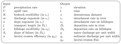
where

t the time, z the soil elevation x the downstream direction and U the uplift rate. ϵ describes the erosion rate in a given point of the river with K an erodibility-rainfall constant, A the drainage area above that given point, m a constant, and S the slope. The term K_diff corresponds to the processes that do not transport material very far (soil creep, animal trails, etc), lumped into a diffusive equation. K_diff is a diffusivity parameter. Both rates, the river incision rate and the hillslope erosion rate are competing processes. If incision rate wins, river can form and grow.

Equation 1 is a kind of diffusion-advection equation. By analogy with fluid mechanics, it is possible to evaluate the relative strength of river and hillslopes processes. The parameter that measures this strength is the non-dimensional Pecklet number, which describes the strength of channel incision relative to soil creep at a chosen scale L:

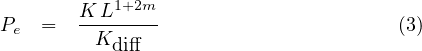
Perron et al. (2012) showed that river branching emerges when Pe > 250. Below this value there are only parallel rivers without tributary forming gentle ripples in the topography. Above this value branching begins to appear and to became stable. Larger P_e thresholds determine the existence of tributaries of tributaries. They showed that this theory was consistent with low relief landscapes in Pennsylvania and California.

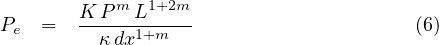
Is this theory consistent with simulations in this website? First let’s compare our equations. In Cidre,

and because n = 1 and the water discharge q = Q∕dx = PA∕dx (dx is pixel size, P precipitation rate - see the Theory page) we can rewrite this equation as

Thus we have the same equation but their ”K” is our ””. We do not develop that here, but their diffusive term is also included in Cidre. Both equations give the same results if their ”K_diff” is our κdx (see Carretier et al., 2016). The difference between Cidre and the Perron’s model is that deposition does occur in rivers in Cidre, and the hillslopes erosion includes the average effect of shallow landslides on steep hillslopes. Nevertheless, we can test the theory based on a simpler model. With our notation, the Pecklet number established by Perron et al. (2012) writes

The characteristic length L is the catchment length (~ 20 km in our simulations). In the reference simulation (m = 0.5), P_e = 141421. Consistently, the drainage network is well developed in planform. In simulation ”Hillslope erodibility x100”, where κ was multiplied by 100, P_e = 1414. There is much less tributaries. In simulation ”Hillslope erodibility x1000”, P_e = 141. The landscape is almost flat and there is no tributary, as predicted by the Perron’s theory because P_e < 250.

Suggestions for teaching
Discuss the possible effect of the simplifications: homogeneous lithology (K and κ), precipitation rate, no vegetation, no groundwater and thus no seepage erosion.
Watch the transient evolution of the simulation ”Hillslope erodibility x1000” and discuss the evolution of the drainage network and its stability in time.
Discuss the possible effect of the deposition term D in Cidre on the Pecklet number.
Discuss the possible effect of the slope threshold S_c (see Theory page) on this analysis.

References

Carretier, S., P. Martinod, M. Reich, and Y. Goddéris (2016), Modelling sediment clasts transport during landscape evolution, Earth Surf. Dynam., 4, 237–251, doi:10.5194/esurf-4-237-2016.
Perron, J. T., P. W. Richardson, K. L. Ferrier, and M. Lapotre (2012), The root of branching river networks, Nature, 492(7427), 100+, doi:10.1038/nature11672.