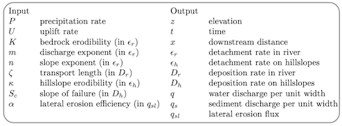
For the experts.

All the following equations and parameters are described in the Theory page.

Intuitively, decreasing the uplift rate may be equivalent to increasing the rainfall rate in terms of mountain height. We can evaluate the equivalence of changing parameters by rewriting the equation in a ”non-dimensional” form. For example, instead of having elevation z we will have z dividing by some constant reference elevation, or a scaling factor, let’s say H, and this will give us z_*, an elevation but without dimension. Its unit is ... an arbitrary unit of elevation. We do that for all the parameters, replace them into the original mass-balance equation and look at the resulting new equation, that will have some universal meaning as all its parameters have an arbitrary unit of length, time etc.

So we start with the initial mass balance equation (cf Theory page.)

Then, with m = 0.5 and n = 1 and using the scaling factors H for mountain height, L for mountain width, P for effective precipitation rate (runoff) and U uplift rate, H∕U for time, we obtain the non-dimensional form (_*) of the mass balance equation 1 (Carretier et al., 2018):

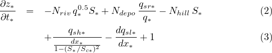
where

N_riv = KU^-1P^0.5L^-0.5H
N_depo = ξ^-1P^-1
N_hill = κHU^-1L^-1

These numbers are called ”non-dimensional numbers” (Rmq. N_depo is G in Guerit et al. (2019) - see the post about the scaling between mountain height and rainfall). These numbers say that for two simulations 1 and 2 with different parameters but such that their non-dimensional numbers are the same, then the evolution of the mean non-dimensional erosion (ϵ₁∕U₁ and ϵ₂∕U₂) over non-dimensional time (t₁ * U₁∕H₁ and t₂ * U₂∕H₂) or the final non-dimensional mountain height (z₁∕H₁ and z₂∕H₂) will be similar. Experts can read Whipple and Tucker (1999).

In particular, let’s imagine two simulations with K₁ = 2K₂ and U₁ = U₂∕2. Then non-dimensional numbers are the same in both cases and it can be predicted that the evolution of the landscape will be similar in both cases. In other words, doubling the erodibility or reducing the uplift rate by 2 have the same effect on the topography. It is moreover a problem to interpret the different altitudes of mountains in terms of tectonic uplift because their erodability is generally unknown.

However, this analysis does not predict everything. For example, the relative effect of U and P is difficult to establish because the parameter chosen for the altitude H, which is the final altitude of the mountain, itself depends on P and U. Similarly, as explained in the post ”The scaling of mountain relief with rainfall”, the relative weight of U and P depends on ζ, the transport length parameter.

Suggestion for teaching:
From dimensionless numbers, predict the equivalence between some parameters and verify this equivalence using the site simulations.
Re-write the non-dimensional equation with other scaling factors and discuss the resulting non-dimensional numbers.

References

Carretier, S., Y. Godderis, J. Martinez, M. Reich, and P. Martinod (2018), Colluvial deposits as a possible weathering reservoir in uplifting mountains, Earth Surface Dynamics, 6(1), 217–237, doi:10.5194/esurf-6-217-2018.
Guerit, L., X.-P. Yuan, S. Carretier, S. Bonnet, S. Rohais, J. Braun, and D. Rouby (2019), Fluvial landscape evolution controlled by the sediment deposition coefficient: Estimation from experimental and natural landscapes, Geology, 47(9), 853–856, doi:10.1130/G46356.1.
Whipple, K. X., and G. E. Tucker (1999), Dynamics of the stream-power incision model: implication for heigth limits of mountain ranges, landscape response timescales, and research needs, J. Geophys. Res., 104, 17,661–17,674.